If you’re using TensorFlow.js to deploy your models to a browser, it’s interesting to take a moment and consider what that model looks like on the inside. In this tutorial, you’re going to take.a look inside a deployed TensorFlow.js model.

First you’ll learn how to convert a model created using python, then you’ll deep dive into the innards of the saved model.

Before we begin, it’s important to note that you can also save a model for use by TensorFlow.js using TensforFlow.js. That is to say, if you use TensorFlow.js to train a model (which you can learn how to do in some of my other tutorials), you can also save your model using the same Javascript API. However, I chose to convert a Python model because I felt like it’s a fairly common task to be given a Python model, and then have to convert it for use in the browser.

In this tutorial, you’ll be using Google Colab. If you need a quick primer on how to get setup, I suggest taking a look at this tutorial. However, feel free to use whatever Python environment you’re comfortable with. Just note, at minimum, you’ll need TensorFlow installed, either version 1.x or 2.x.

Creating the Python Model Using Python, you’ll first create a very simple model, meant to predict a linear function, specifically y = 2 * x - 1. In a free cell, add the following code to train the model:

import numpy as np
import tensorflow as tf
from tensorflow import keras
print(tf.__version__)
model = tf.keras.Sequential([keras.layers.Dense(units=1, input_shape=[1])])
model.compile(optimizer='sgd', loss='mean_squared_error')
xs = np.array([-1.0, 0.0, 1.0, 2.0, 3.0, 4.0], dtype=float)
ys = np.array([-3.0, -1.0, 1.0, 3.0, 5.0, 7.0], dtype=float)
model.summary()
model.fit(xs, ys, epochs=500)

Note: At the time of writing this tutorial. the default version of TensorFlow is 2.1.0.

Nothing too exciting in the above code. You create a Sequential model with a single Dense layer, taking in a single value, and outputting a single value. You use stochastic gradient descent (sgd) and the mean squared error (mse) to train the model. You create a very limited training dataset, and train your model for 500 epochs.

Looking at the summary of the model, you’ll see that your model has 2 trainable params (1 note and 1 bias). Your output should look something like this:

Model: "sequential"
_________________________________________________________________
Layer (type)                 Output Shape              Param #   
=================================================================
dense (Dense)                (None, 1)                 2         
=================================================================
Total params: 2
Trainable params: 2
Non-trainable params: 0
_________________________________________________________________

If you’re curious how well your model does, feel free to run a quick test prediction using the following code:

print(model.predict([10.0]))

Before you can convert this model for use by TensorFlow.js, you’ll first need to save the model to disk. Use the following code to save the model. Depending on the version of TensorFlow you have running, you may have to un-comment the code the code that works for you

import time
saved_model_path = f"/tmp/saved_model/{int(time.time())}"

# for TensorFlow 2.0
tf.saved_model.save(model, saved_model_path)

# for TensorFlow 1.x
# tf.contrib.saved_model.save_keras_model(model, saved_model_path)

Note the path of the saved file. In my case, the path to the saved model is /tmp/saved_model/1587980957/.

Ok, with a Python model done, it’s time to convert this bad boy for TensorFlow.js

Converting the Model for TensorFlow.js

In order to convert your model, you’ll need to install the tensorflowjs_converter tool, which is part of the TensorFlow.js library. Run the following command in a free cell inside Colab

!pip install tensorflowjs

Note: I actually get a bunch of warnings and errors when trying to install that python package, but it alls seems to work regardless 🤷🏽‍♂️.

Finally, convert your model using the following command, making sure to replace the path to the model with the path to your own model

!tensorflowjs_converter --input_format=keras_saved_model /tmp/saved_model/1587980957 /tmp/linear

This should generate two files inside the /tmp/linear folder. Namely model.json and group1-shard1of1.bin.

In the proceeding sections, we’ll dive a little bit into what’s in those files, but before we do that, it’s important to know how to load your model to perform inference.

TensorFlow.js provides a few ways to load your model, using the same loadLayersModel API. My guess is, most developers will load models over HTTPS. This means that you would pass a URL into loadLayersModel pointing to the model.json file.

const model = await tf.loadLayersModel('http://model-server.domain/download/model.json');

Note: TensorFlow.js will attempt to load the subsequent group*-shard*of*.bin files assuming they’re in the same directory.

Ok with that little tangent out the way, time to take a peek inside those saved models

Reading model.json

Since the model.json file is the file served to loadLayersModel, it’s a good place to start breaking things down. Open the file using any text editor. You should see something as follows:

{
  "format":"layers-model",
  "generatedBy":"keras v2.2.4-tf",
  "convertedBy":"TensorFlow.js Converter v1.7.3",
  "modelTopology": {...},
  "weightsManifest": [...]
}

Nothing too interesting here. It’s nice to know which version of the tools where used when generating the model, so you can always go back and compare any differences, however I sincerely doubt these are used anywhere. The more interesting properties seem to be the modelTopology and the weightsManifest. You’ll look at each of these sections in turn, starting with the modelTopology.

"modelTopology": {
     "keras_version":"2.2.4-tf",
     "backend":"tensorflow",
     "model_config":{...}
     "training_config":{...}
}

Pretty straight forward, the topology contains the model_config and the training_config. If you look at the contents of training_config, you’ll notice that the model remembers the loss and the optimizer used for training. Not super interesting unless you want to compare two models, and how they were trained. You should see something that looks as follows:

"training_config":{
  "loss":"mean_squared_error",
  "metrics":[

  ],
  "weighted_metrics":null,
  "sample_weight_mode":null,
  "loss_weights":null,
  "optimizer_config":{
    "class_name":"SGD",
    "config":{
    "name":"SGD",
    "learning_rate":0.009999999776482582,
    "decay":0.0,
    "momentum":0.0,
    "nesterov":false
    }
  }
}

The model_config is slightly more interesting, since you’re able to parse the way the model is architected. This is very useful if you’re going to do transfer learning with your models. In your case, you should see something like this:

"model_config":{
  "class_name":"Sequential",
  "config":{
    "name":"sequential",
    "layers":[...]
  }
}

Immediately, you can see that this is a Sequential Keras model. Peeking inside the layers of this object you’ll see some other interesting properties:

"layers":[{
  "class_name":"Dense",
  "config":{
    "name":"dense",
    "trainable":true,
    "batch_input_shape":[ null, 1 ],
    "dtype":"float32",
    "units":1,
    "activation":"linear",
    "use_bias":true,
    "kernel_initializer":{
      "class_name":"GlorotUniform",
      "config":{ "seed":null }
    },
    "bias_initializer":{
      "class_name":"Zeros",
      "config":{}
    },
    "kernel_regularizer":null,
    "bias_regularizer":null,
    "activity_regularizer":null,
    "kernel_constraint":null,
    "bias_constraint":null
  }
}]

Again, you can see the how the model was constructed. In our case, it’s trivial since we created the model, however, in the case where you may just be given the saved model, or want to see someone else’s TensorFlow.js saved model, it’s interesting to be able to see how it was constructed.

The most important piece of information here is the name of the layer inside the “config” property. In this case, the name is “dense”, and it’s the value used when looking at the weightsManifest.

Dumping the contents of the weightsManifest, you can see some more interesting stuff

"weightsManifest":[{
  "paths":["group1-shard1of1.bin"],
  "weights":[{
    "name":"dense/kernel",
    "shape":[1, 1],
    "dtype":"float32"
  }, {
    "name":"dense/bias",
    "shape":[1],
    "dtype":"float32"
  }]
}]

The last bit of information here is the path to the binary weights file. Since our model is fairly small, there’s only one shard needed to represent the weights of this model. However, if you were curious to how the converter decides how many files to create to store the weights, look no further than write_weights.py in the github repository. I’ll just post the comment from the write_weights method here:

Writes weights to a binary format on disk for ingestion by JavaScript.

Weights are organized into groups. When writing to disk, the bytes from all weights in each group are concatenated together and then split into shards (default is 4MB). This means that large weights (> shard_size) get sharded and small weights (< shard_size) will be packed. If the bytes can’t be split evenly into shards, there will be a leftover shard that is smaller than the shard size.

Weights are optionally quantized to either 8 or 16 bits for compression, which is enabled via the quantization_dtype argument.

Pretty interesting stuff!

At this point, you know more about model.json than you probably thought was necessary. Now it’s time to turn your attention to the weight file.

Understanding the Binary Weights File If you open up the group1-shard1of1.bin in any editor, it should look like garbage. However, if you open the file using a hex viewer (I’m currently using hexdump for VSCode). You should see something like as follows:

Ok, so you know this is binary, and you know you should have 2 weights (1 for the kernel/node and one for the bias). If you don’t want to bother deciphering the binary directly, you can go back to your model and dump the values of the weights first

model.get_layer(index=0).get_weights()

You should get an output that looks as follows (your values will be different based on what data, and how long your trained your model)

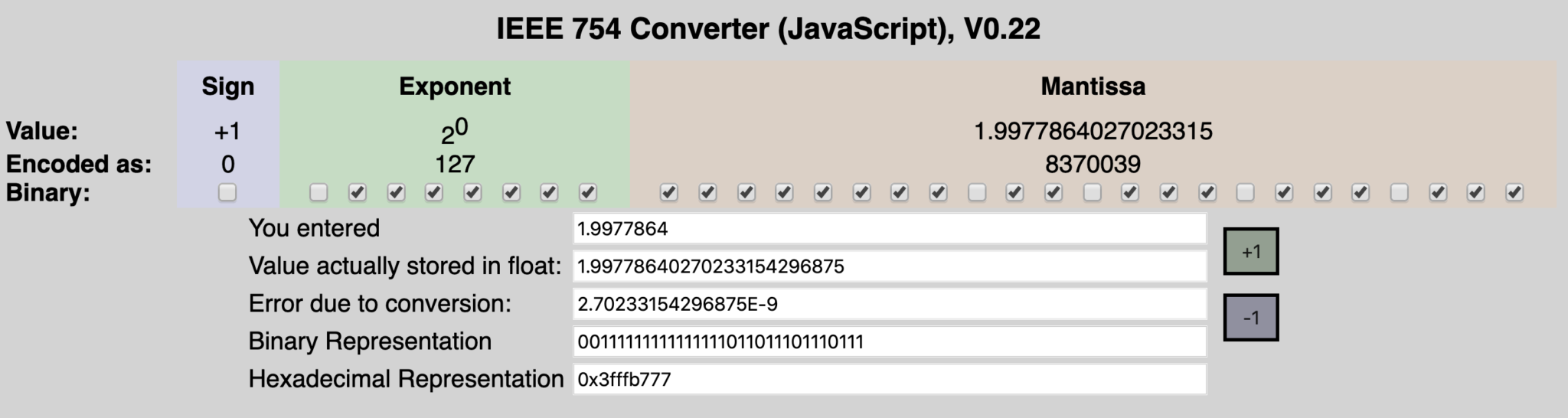
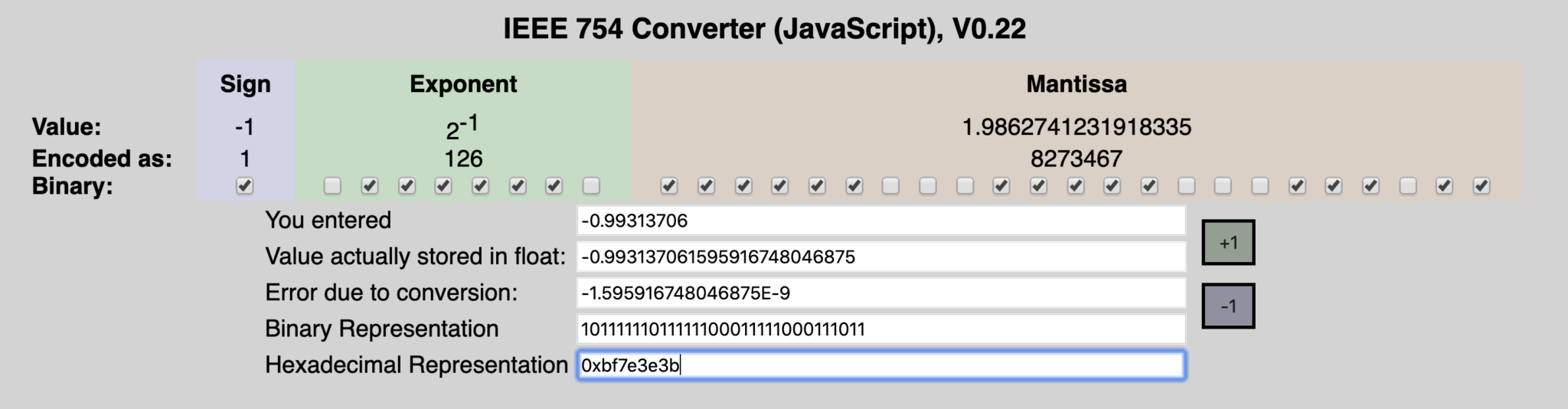
[array([[1.9977864]], dtype=float32), array([-0.99313706], dtype=float32)]

Recall that the data you pass in approximates y = 2x - 1. The values we get from our model are close but not exact to 2, and -1.

You can use any trusty IEEE-754 Floating point converter to convert the floating points values. Here’s what I got:

If you’re interested in how to convert from floating point to hex or binary, you should checkout this link, it’s pretty nerdy, but if you like 0’s and 1’s, its a great read.

Ok! So it looks like, the converter stores the weights using Little Endian when writing to the weights file. It also seems that, based on the arguments passed into the converter, the weights are quantized to 8 bits by default.

Takeaways

And that’s it. Digging into the model files used by TensorFlow.js can be a boring chore, but it can be important when dealing with converting between platforms.